Dimension Reduction
Dimension reduction is a crucial step in data preprocessing that serves several key purposes in data analysis and machine learning. By reducing the number of input variables in a dataset, dimension reduction techniques help to simplify the data while retaining its essential structure. This process is particularly important for several reasons:
Noise Reduction: High-dimensional data often contains noise and irrelevant information that can obscure the underlying patterns. Dimension reduction helps to filter out this noise, making it easier to identify the true structure of the data.
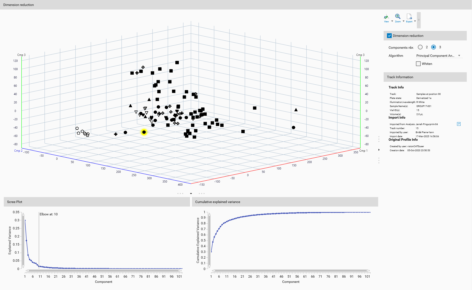
Visualization: High-dimensional data is difficult to visualize and interpret. Dimension reduction techniques can project the data into a lower-dimensional space, in this case three dimensions, making it easier to create meaningful visualizations. This can aid in exploratory data analysis and help to identify patterns and relationships within the data. Display will always display the tracks processed by the dimension reduction algorithm (more specifically, the position in the 3D space (or 2D space), not the colors).
Feature Extraction: Dimension reduction can also serve as a feature extraction method, where the reduced dimensions represent new features that capture the most important information in the data. These new features can be more informative and easier to work with than the original set of variables. Therefore, dimension reduction can make the data more interpretable.
Important
Dimension reduction is only available when the Unsupervised classification mode is selected in Classification mode.
Activation
Dimension reduction can be enabled by checking the checkbox. It is an optional step that can be used to preprocess the data before applying unsupervised algorithms.
Components number
The number of components to keep can be set in the Components nbr. field. It must be at least 2 to be able to visualize the data in 2D or 3D. To allow a meaningful visualization, the maximum number of components is limited to 3.
Dimension Reduction Algorithms
Several dimension reduction algorithms are available:
Principal Component Analysis (PCA)
PCA is a statistical procedure that uses an orthogonal transformation to convert a set of observations of possibly correlated variables into a set of values of linearly uncorrelated variables.
Parameters
Whiten: Whitening is a preprocessing step that transforms the data to have the identity matrix as its covariance matrix. This can help in improving the performance of PCA by ensuring that all features contribute equally to the analysis.
Helpers
Scree Plot
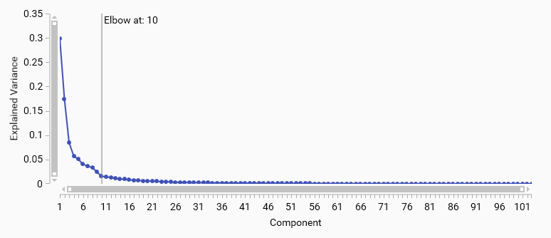
A PCA scree plot shows the variance explained by each principal component in descending order; the “elbow” is the point where the curve changes from steep to flat and indicates diminishing returns from additional components. Components up to the elbow typically capture the main signal.
Use the elbow as a starting choice, then confirm with the cumulative variance (e.g., 70–95% depending on the task) . If no clear elbow appears, prefer explained‑variance thresholds.
Cumulative Explained variance
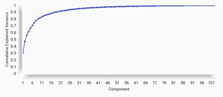
A cumulative explained variance plot shows the total variance explained by the first N principal components. It helps to determine how many components are needed to capture a desired amount of variance in the data.
For example, if you want to retain 90% of the variance, you can look for the point on the curve where the cumulative explained variance reaches 0.9 and select that number of components.
Kernel Principal Component Analysis (PCA)
Kernel PCA extends Principal Component Analysis by incorporating kernel methods, enabling nonlinear dimensionality reduction.
Parameters
Kernel: The kernel function defines the type of transformation applied to the data. Different kernels can capture different types of relationships in the data.
Linear
Polynomial
Radial Basis Function (Rbf)
Sigmoid
Cosine
Sliced Wasserstein Distance
Note
Sliced Wasserstein Distance is computationally expensive and may not be suitable for large datasets. Therefore, it is only available in Peaks Data Mode.
Gamma: Gamma defines the influence of individual training examples. It is only applicable to the Rbf kernel. Possible values include:
Auto: \(\frac{1}{n_{\text{features}}}\) A gamma value that is inversely proportional to the number of features, providing a baseline scaling.
a custom value: A user-defined gamma value that can be set to tailor the model’s sensitivity to the data distribution.
t-Distributed Stochastic Neighbor Embedding (t-SNE)
t-SNE is a machine learning algorithm for dimensionality reduction particularly well-suited for the visualization of high-dimensional datasets.
Parameters
Perplexity: Perplexity is a parameter that affects the balance between local and global aspects of the data. It can be thought of as a measure of the effective number of neighbors. A smaller perplexity focuses more on local structure, while a larger perplexity captures more global structure.
Possible values range from \(1\) to \({n_{\text{features}}} - 1\), with common choices being 30 or 40 for many datasets.
A smaller perplexity (e.g., 5-20) is often used for datasets with a lot of local structure, while larger values (e.g., 30-50) are better for datasets where global structure is more important.
Important
The perplexity value should be chosen based on the specific characteristics of the dataset and the desired balance between local and global structure. A wrong choice will lead to poor results, such as clusters that are too tight or too scattered.
Learning Rate: The learning rate determines how quickly the algorithm adapts to the data. A higher learning rate can lead to faster convergence but may overshoot the optimal solution, while a lower learning rate can result in more stable convergence but may take longer.
Max. Iterations: The maximum number of iterations specifies how many times the algorithm will update the embedding. More iterations can lead to better convergence but will take longer to compute.
Uniform Manifold Approximation and Projection (UMAP)
UMAP is a dimension reduction technique that can capture more of the global data structure compared to t-SNE.
Parameters
Neighborhood Size: Neighborhood size is a key parameter that determines how many nearest neighbors are considered when constructing the manifold approximation. It affects the balance between local and global structure in the data.
Smaller values (e.g., 5-15) will focus more on local structure, capturing fine-grained relationships between points.
Larger values (e.g., 30-50) will capture more global structure, allowing for broader relationships to be represented in the embedding.
Minimum Distance: Minimum distance is a parameter that controls how tightly UMAP is allowed to pack points together in the low-dimensional representation. It affects the spacing between points in the embedding.
Smaller values (e.g., 0.001-0.5) will result in a more clustered embedding, where points are packed closely together.
Larger values (e.g., 0.5-100) will result in a more spread-out embedding, allowing for more space between points.
Sparse Principal Component Analysis (PCA)
Sparse PCA is a variant of PCA that introduces sparsity into the input variables. This can make the model easier to interpret by reducing the number of non-zero components.
Parameters
Alpha: is a parameter that controls the sparsity of the solution. Higher values of alpha will result in sparser solutions.
Display
A 3D view is available to visualize the samples in the reduced space, either 2D or 3D depending on number of components selected. It will help to understand the effect of the dimension reduction algorithm on your data.
General 3D View features are explained in the Profiles viewer section.
Toolbar
General 3D View tools are explained in the Profiles viewer section.
Track Information
A track can be selected either from the Overview or from the Display. The details of the selected track are then displayed here, like in Track information.