Unsupervised Classification
Unsupervised classification groups data without prior knowledge of the class labels. It is used to identify inherent structures or patterns in the data by clustering similar data points together based on their features.
Important
The defined classes, via Class labeling, as seen in Overview, are not used in unsupervised classification. Instead, the algorithm identifies clusters based on the data’s characteristics. But if classes were previously defined, they will still be displayed in Overview and the corresponding markers will appear in the 2D or 3D views.
Important
Unsupervised classification works on either on original or reduced dataset, as defined in the Dimension Reduction section. Therefore, it is critical to select the appropriate dimension reduction algorithm before applying unsupervised classification.
Unsupervised Classification Algorithms
Unsupervised classification techniques are used to identify inherent groupings in the data without prior labels.
Several dimension reduction algorithms are available:
K-means
K-means is a centroid-based algorithm that aims to partition n observations into k clusters in which each observation belongs to the cluster with the nearest mean.
Parameters
Max. clusters: The maximum number of clusters to form as well as the maximum number of centroids to generate. This parameter defines how many distinct groups the algorithm will attempt to identify in the data.
Nbr. classes: Sets the maximum number of clusters to the number of defined classes in the Overview section.
Custom: Allows the user to specify a custom number of clusters.
Distance: The metric used to compute the distance between data points and cluster centroids.
Euclidean: The straight-line distance between two points in Euclidean space.
Manhattan: The distance between two points measured along axes at right angles, also known as the L1 norm.
Cosine: Measures the cosine of the angle between two vectors, often used in text analysis to measure document similarity.
Mahalanobis: Takes into account the correlations of the data set and is scale-invariant.
Wasserstein: Also known as Earth Mover’s Distance, used in optimal transport theory to measure the distance between probability distributions.
Helpers
K-means elbow
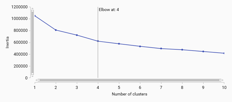
K-means elbow method helps to determine the optimal number of clusters by plotting the explained variance as a function of the number of clusters. The “elbow” point in the plot indicates the optimal number of clusters where adding more clusters does not significantly improve the model.
Average silhouette score vs. number of clusters
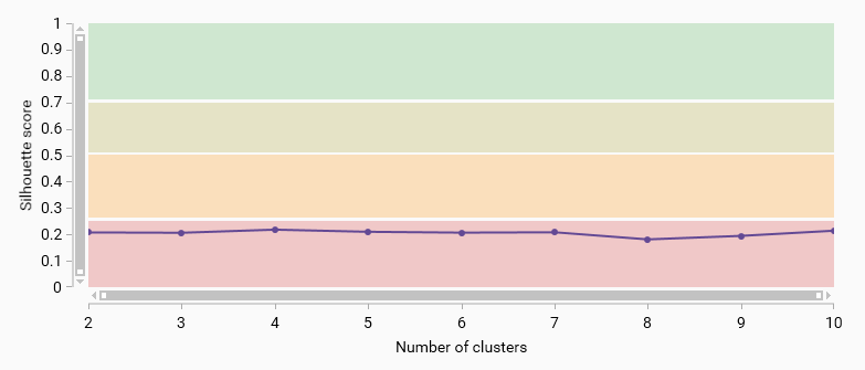
The average silhouette score measures how similar an object is to its own cluster compared to other clusters. A higher silhouette score indicates better-defined clusters. This plot helps to evaluate the quality of clustering for different numbers of clusters.
Four color bands indicate the quality of the clustering: - 0.71 - 1.00: Strong structure has been found. - 0.51 - 0.70: Reasonable structure has been found. - 0.26 - 0.50: Weak structure has been found - 0.00 - 0.25: No substantial structure has been found.
Density-Based Spatial Clustering of Applications with Noise (DBSCAN)
DBSCAN is a density-based clustering algorithm that groups together points that are close to each other based on a distance measurement and a minimum number of points.
Parameters
Epsilon: The maximum distance between two points for one to be considered as in the neighborhood of the other. This parameter influences the size of the clusters; a smaller epsilon value will result in smaller clusters.
Min. Samples: The minimum number of points required to form a dense region. For a point to be considered a core point (and thus form part of a cluster), it must have at least Min. Samples within its epsilon neighborhood. This parameter influences the density of the clusters; a higher value will result in more points being classified as noise.
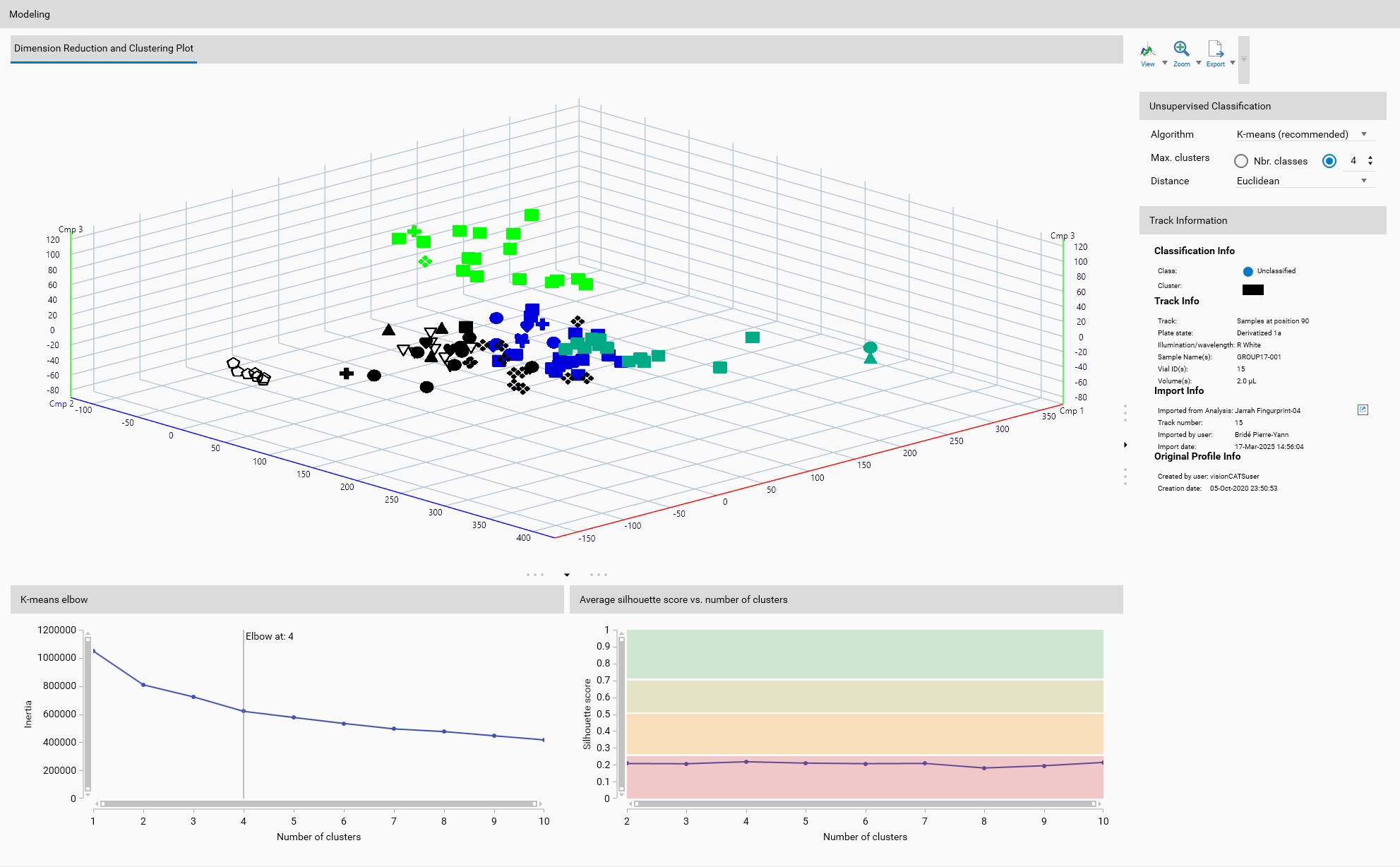
Display
The 3D View will show each cluster in a different color, allowing for visual differentiation of the clusters.
General 3D View features are explained in the Profiles viewer section.
Toolbar
General 3D View tools are explained in the Profiles viewer section.
Track Information
A track can be selected either from the Overview or from the Display. The details of the selected track are then displayed here, like in Track information.